Heat distance, transport, & logarithmic map on point clouds

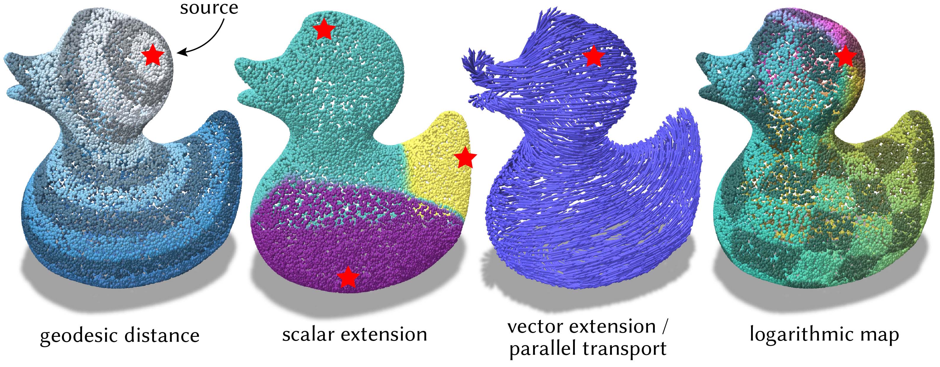
Compute signed and unsigned geodesic distance, transport tangent vectors, and generate a special parameterization called the logarithmic map using fast solvers based on short-time heat flow.

point cloud heat solve results

These routines implement point cloud versions of the algorithms from:

The Heat Method for Distance Computation (distance)
The Vector Heat Method (parallel transport and log map)
A Heat Method for Generalized Signed Distance (signed distance)
A Laplacian for Nonmanifold Triangle Meshes (used to build point cloud Laplacian for all)

All computation is encapsulated by the PointCloudHeatSolver class, which maintains prefactored linear systems for the various methods. Some setup work is performed both on construction, and after the first query. Subsequent queries, even with different source points, will be fast.

#include "geometrycentral/pointcloud/point_cloud_heat_solver.h"

Example: Basic usage

#include "geometrycentral/pointcloud/point_cloud.h"
#include "geometrycentral/pointcloud/point_position_geometry.h"
#include "geometrycentral/pointcloud/point_cloud_heat_solver.h"
#include "geometrycentral/pointcloud/point_cloud_io.h"

using namespace geometrycentral;
using namespace geometrycentral::pointcloud;

// Read in a point cloud
std::unique_ptr<PointCloud> cloud;
std::unique_ptr<PointPositionGeometry> geom;
std::tie(cloud, geom) = readPointCloud("my_cloud.ply");

// Create the solver
PointCloudHeatSolver solver(*cloud, *geom);

// Pick a source point or two
Point pSource = cloud->point(7);
Point pSource2 = cloud->point(8);

// Pick a source curve or two
std::vector<std::vector<Point>> curves;
curves.push_back({cloud->point(11), cloud->point(12), cloud->point(15), cloud->point(14), cloud->point(13)});
curves.push_back({cloud->point(17), cloud->point(18), cloud->point(19)});

// Compute geodesic distance
PointData<double> distance = solver.computeDistance(pSource);

// Compute signed distance to a set of curves.
PointData<double> signedDistance = solver.computeSignedDistance(curves, pointNormals);

// Compute scalar extension
PointData<double> extended = solver.extendScalars({{pSource,  3.},
                                                   {pSource2, -5.}});

// Compute parallel transport
Vector2 sourceVec{1, 2};
PointData<Vector2> transport = solver.transportTangentVector(pSource, sourceVec);

// Compute the logarithmic map
PointData<Vector2> logmap = solver.computeLogMap(pSource);

Constructor

PointCloudHeatSolver::PointCloudHeatSolver(PointCloud& cloud, PointPositionGeometry& geom, double tCoef = 1.0)

Create a new solver for the heat methods. Precomputation is performed at startup and lazily as needed.

cloud is the point cloud to operate on.
geom is the geometry (e.g., vertex positions) for the cloud. Note that nearly any point cloud geometry object can be passed here. For instance, use a PointPositionFrameGeometry if you want to represent tangent-valued data in tangent bases of your own choosing.
tCoef is the time to use for short time heat flow, as a factor m * h^2, where h is the mean between-point spacing. The default value of 1.0 is almost always sufficient.

Algorithm options (like tCoef) cannot be changed after construction; create a new solver object with the new settings.

Geodesic distance

Geodesic distance is the distance from a given source along the surface represented by the point cloud. Specifying multiple source points yields the distance to the nearest source.

PointData<double> PointCloudHeatSolver::computeDistance(const Point& sourcePoint)

Compute the geodesic distance from sourcePoint to all other points.

PointData<double> PointCloudHeatSolver::computeDistance(const std::vector<Point>& sourcePoints)

Like above, but for multiple source points.

Signed geodesic distance

PointData<double> computeSignedDistance(const std::vector<std::vector<Point>>& curves, const PointData<Vector3>& cloudNormals, const SignedHeatOptions& options = SignedHeatOptions())

Compute the signed geodesic distance from a set of curves curves to all other points. Each curve in curves is a single connected component specified as a sequence of points; curve normals are determined using the normals of the point cloud, specified using cloudNormals.

The SignedHeatOptions struct allows several options:

Field	Default value	Meaning
`bool preserveSourceNormals`	`false`	If `true`, preserve the initial curve normals at the source curve during vector diffusion.
`LevelSetConstraint levelSetConstraint`	`LevelSetConstraint::ZeroSet`	Specifies how/if level sets should be preserved. Can be set to `LevelSetConstraint::ZeroSet`, `LevelSetConstraint::Multiple`, or `LevelSetConstraint::None`, corresponding to preserving the zero set, mulitple level sets (one for each curve component), or no level sets, respectively.
`double softLevelSetWeight`	`-1`	If greater than 0, gives the weight with which the given level set constraint is “softly” enforced.

Scalar extension

Given scalar values defined at isolated points in the cloud, extend it to a scalar field on all points. Each point will take the value from the nearest source point, in the sense of geodesic distance. Note that the fast diffusion algorithm means the result is a slightly smoothed-out field.

PointData<double> PointCloudHeatSolver::extendScalars(const std::vector<std::tuple<Point, double>>& sources)

Given a collection of source points and scalars at those points, extends the scalar field to the whole cloud as a nearest-geodesic-neighbor interpolant.

Vector extension

Given tangent vectors defined at one or more isolated source locations on a surface, extend transport the vectors across the entire domain according to parallel transport. Each point on the domain will take the value of the nearest source point. Note that the fast diffusion algorithm means the result is a slightly smoothed-out field.

Despite operating on tangent-valued data, these routines work as expected even on a point cloud with inconsistent normal orientations. See connection Laplacian for more details.

PointData<Vector2> PointCloudHeatSolver::transportTangentVector(const Point& sourcePoint, const Vector2& sourceVector)

Shorthand for the general version below when there is just one vector.

Computes parallel transport of the given vector along shortest geodesics to the rest of the cloud.

Polar directions are defined in each point’s tangent space. See PointPositionGeometry::tangentBasis.

PointData<Vector2> PointCloudHeatSolver::transportTangentVectors(const std::vector<std::tuple<Point, Vector2>>& sources)

Given a collection of source points and tangent vectors at those points, extends the vector field to the whole cloud as a nearest-geodesic-neighbor interpolant via parallel transport along shortest geodesics.

Polar directions are defined in each point’s tangent space. See PointPositionGeometry::tangentBasis.

Logarithmic Map

The logarithmic map is a very special 2D local parameterization of a surface about a point, where for each point on the surface the magnitude of the log map gives the geodesic distance from the source, and the polar coordinate of the log map gives the direction at which a geodesic must leave the source to arrive at the point.

Despite operating on tangent-valued data, this routine works as expected even on a point cloud with inconsistent normal orientations. See connection Laplacian for more details.

PointData<Vector2> PointCloudHeatSolver::computeLogMap(const Point& sourcePoint)

Computes the logarithmic map from the given source point.

Polar directions are defined in each point’s tangent space. See PointPositionGeometry::tangentBasis.